Stuff

Links

Dependent Types in Haskell: Binomial Heaps 101

Haskell eXchange

Update: I gave a talk about this blogpost at the Haskell eXchange 2018 on the 11th of October 2018. You can watch the video here. Note that you will need to create an account in on the skillsmatter website in order to watch the recording.

Introduction

This post makes a bit of a departure from the “practical Haskell” I usually try to write about, although – believe it or not – this blogpost actually originated from a very practical origin ¹.

This blogpost is a literate Haskell file, which means you can just download it here and load it into GHCi to play around with it. In this case, you can also verify the properties we will be talking about (yes, GHC as a proof checker). Since we are dipping our toes into dependent types territory here, we will need to enable some extensions that are definitely a bit more on the advanced side.

{-# LANGUAGE DataKinds            #-}
{-# LANGUAGE GADTs                #-}
{-# LANGUAGE KindSignatures       #-}
{-# LANGUAGE PolyKinds            #-}
{-# LANGUAGE ScopedTypeVariables  #-}
{-# LANGUAGE TypeFamilies         #-}
{-# LANGUAGE TypeOperators        #-}
{-# LANGUAGE UndecidableInstances #-}

Since the goal of this blogpost is mainly educational, we will only use a few standard modules and generally define things ourselves. This also helps us to show that there is no magic going on behind the scenes: all term-level functions in this file are total and compile fine with -Wall.

import           Data.List          (intercalate, minimumBy)
import           Data.List.NonEmpty (NonEmpty (..))
import qualified Data.List.NonEmpty as NonEmpty
import           Data.Ord           (comparing)

I assume most readers will be at least somewhat familiar with the standard length-indexed list:

data Nat = Zero | Succ Nat deriving (Show)

data Vec (n :: Nat) a where
    VNull :: Vec 'Zero a
    VCons :: a -> Vec n a -> Vec ('Succ n) a

These vectors carry their length in their types. In GHCi:

*Main> :t VCons "Hello" (VCons "World" VNull)
Vec ('Succ ('Succ 'Zero)) [Char]

This blogpost defines a similar way to deal with binomial heaps. Binomial heaps are one of my favorite data structures because of their simple elegance and the fascinating way their structure corresponds to binary numbers.

We will combine the idea of Peano number-indexed lists with the idea that binomial heaps correspond to binary numbers to lift binary numbers to the type level. This is great because we get O(log(n)) size and time in places where we would see O(n) for the Peano numbers defined above (in addition to being insanely cool). In GHCi:

*Main> :t pushHeap 'a' $ pushHeap 'b' $ pushHeap 'c' $
            pushHeap 'd' $ pushHeap 'e' emptyHeap
Heap ('B1 ('B0 ('B1 'BEnd))) Char

Where 101 ² is, of course, the binary representation of the number 5.

Conveniently, 101 also represents the basics of a subject. So the title of this blogpost works on two levels, and we present an introductory-level explanation of a non-trivial (and again, insanely cool) example of dependent Haskell programming.

Table of contents

1. Introduction
2. Singletons and type equality
3. Binomial heaps: let’s build it up
   1. Binomial trees
   2. Type level binary numbers
   3. Binomial forests
   4. The binomial heap
4. Binomial heaps: let’s break it down
   1. Taking apart a single tree
   2. More Vec utilities
   3. Popcount and width
   4. Lumberjack
   5. Lumberjack: final form
   6. popHeap: gluing the pieces together
5. Acknowledgements
6. Appendices
   1. Appendix 1: runtime cost of this approach
   2. Appendix 2: “pretty”-printing of heaps
   3. Appendix 3: left-to-right increment

Singletons and type equality

If I perform an appropriate amount of hand-waving and squinting, I feel like there are two ways to work with these stronger-than-usual types in Haskell. We can either make sure things are correct by construction, or we can come up with a proof that they are in fact correct.

The former is the simpler approach we saw in the Vec snippet: by using the constructors provided by the GADT, our constraints are always satisfied. The latter builds on the singletons approach introduced by Richard Eisenberg and Stephanie Weirich.

We need both approaches for this blogpost. We assume that the reader is somewhat familiar with the first one and in this section we will give a brief introduction to the second one. It is in no way intended to be a full tutorial, we just want to give enough context to understand the code in the blogpost.

If we consider a closed type family for addition of natural numbers (we are using an N prefix since we will later use B for addition of binary numbers):

type family NAdd (x :: Nat) (y :: Nat) :: Nat where
    NAdd ('Succ x) y = 'Succ (NAdd x y)
    NAdd 'Zero     y = y

We can trivially define the following function:

data Proxy a = Proxy

cast01 :: Proxy (NAdd 'Zero x) -> Proxy x
cast01 = id

NAdd 'Zero x is easily reduced to x by GHC since it is simply a clause of the type family, so it accepts the definition id. However, if we try to write

cast02 :: Proxy (NAdd x 'Zero) -> Proxy x
cast02 = id

We run into trouble, and GHC will tell us:

Couldn't match type ‘x’ with ‘NAdd x 'Zero’

We will need to prove to GHC that these two types are equal – commutativity doesn’t come for free! This can be done by providing evidence for the equality by way of a GADT constructor ³.

data EqualityProof (a :: k) (b :: k) where
    QED :: EqualityProof a a

type a :~: b = EqualityProof a b

Take a minute to think about the implications this GADT has – if we can construct a QED value, we are actually providing evidence that the two types are equal. We assume that the two types (a and b) have the same kind k ⁴.

The QED constructor lives on the term-level though, not on the type-level. We must synthesize this constructor using a term-level computation. This means we need a term-level representation of our natural numbers as well. This is the idea behind singletons and again, a much better explanation is available in said paper and some talks, but I wanted to at least provide some intuition here.

The singleton for Nat is called SNat and it’s easy to see that each Nat has a unique SNat and the other way around:

data SNat (n :: Nat) where
    SZero :: SNat 'Zero
    SSucc :: SNat n -> SNat ('Succ n)

We can use such a SNat to define a proof for what we are trying to accomplish. Since this proof can be passed any n in the form of an SNat, it must be correct for all n.

lemma1 :: SNat n -> NAdd n 'Zero :~: n

GHC can figure out the base case on its own by reducing NAdd 'Zero 'Zero to 'Zero:

lemma1 SZero = QED

And we can use induction to complete the proof. The important trick here is that in the body of the pattern match on EqualityProof a b, GHC knows that a is equal to b.

lemma1 (SSucc n) = case lemma1 n of QED -> QED

This can be used to write cast02:

cast02 :: SNat x -> Proxy (NAdd x 'Zero) -> Proxy x
cast02 snat = case lemma1 snat of QED -> id

cast02 takes an extra parameter and there are several ways to synthesize this value. The common one is a typeclass that can give us an SNat x from a Proxy x. In this blogpost however, we keep things simple and make sure we always have the right singletons on hand by passing them around in a few places. In other words: don’t worry about this for now.

Binomial heaps: let’s build it up

Binomial trees

A binomial heap consists of zero or more binomial trees. I will quote the text from the Wikipedia article here since I think it is quite striking how straightforward the definition translates to GADTs that enforce the structure:

• A binomial tree of order 0 is a single node
• A binomial tree of order k has a root node whose children are roots of binomial trees of orders k−1, k−2, …, 2, 1, 0 (in this order).

data Tree (k :: Nat) a where
    Tree :: a -> Children k a -> Tree k a

data Children (k :: Nat) a where
    CZero :: Children 'Zero a
    CCons :: Tree k a -> Children k a -> Children ('Succ k) a

Some illustrations to make this a bit more clear:

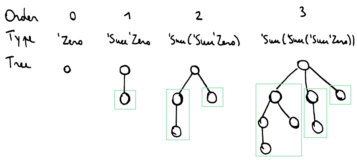
This is definitely a very good example of the correctness by construction approach I talked about earlier: it is simply impossible to create a tree that does not have the right shape.

Empty trees do not exist according to this definition. A singleton tree is easy to create:

singletonTree :: a -> Tree 'Zero a
singletonTree x = Tree x CZero

We only need to define one operation on trees, namely merging two trees.

A tree of order k has 2ᵏ elements, so it makes sense that merging two trees of order k creates a tree of order k+1. We can see this in the type signature as well:

mergeTree :: Ord a => Tree k a -> Tree k a -> Tree ('Succ k) a

Concretely, we construct the new tree by taking either the left or the right tree and attaching it as new child to the other tree. Since we are building a heap to use as a priority queue, we want to keep the smallest element in the root of the new tree.

mergeTree l@(Tree lroot lchildren) r@(Tree rroot rchildren)
    | lroot <= rroot = Tree lroot (CCons r lchildren)
    | otherwise      = Tree rroot (CCons l rchildren)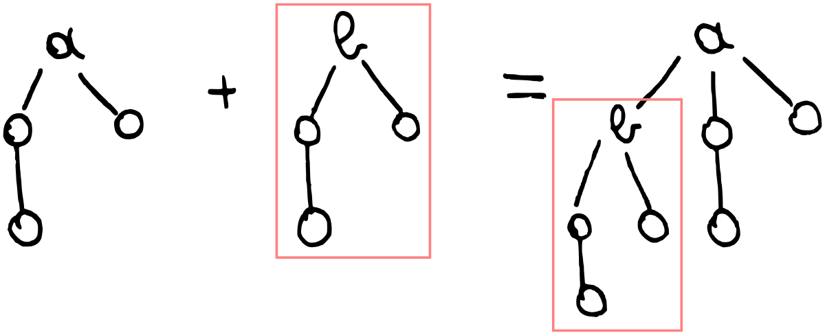

Type level binary numbers

With these trees defined, we can move on to binomial heaps.

While binomial trees are interesting on their own, they can really only represent collections that have a number of elements that are exactly a power of two.

Binomial heaps solve this in a surprisingly simple way. A binomial heap is a collection of binomial trees where we may only have at most one tree for every order.

This is where the correspondence with binary numbers originates. If we have a binomial heap with 5 elements, the only way to do this is to have binomial trees of orders 2 and 0 (2² + 2⁰ = 5).

We start out by defining a simple datatype that will be lifted to the kind-level, just as we did with Nat:

data Binary
    = B0 Binary
    | B1 Binary
    | BEnd
    deriving (Show)

It’s important to note that we will represent binary numbers in a right-to-left order since this turns out to match up more naturally with the way we will be defining heaps.

For example, the type:

'B0 ('B1 ('B1 'BEnd))

represents the number 6 (conventionally written 110).

I think it is fairly common in Haskell for a developer to play around with different ways of representing a certain thing until you converge on an elegant representation. This is many, many times more important when we are dealing with dependently-typed Haskell.

Inelegant and awkward data representations can make term-level programming clunky. Inelegant and awkward type representations can make type-level programming downright infeasible due to the sheer amount of lemmas that need to be proven.

Consider the relative elegance of defining a type family for incrementing a binary number that is read from the right to the left:

type family BInc (binary :: Binary) :: Binary where
    BInc 'BEnd        = 'B1 'BEnd
    BInc ('B0 binary) = 'B1 binary
    BInc ('B1 binary) = 'B0 (BInc binary)

Appendix 3 contains an (unused) implementation of incrementing left-to-right binary numbers. Getting things like this to work is not too much of a stretch these days (even though GHC’s error messages can be very cryptic). However, due to the large amount of type families involved, proving things about it presumably requires ritually sacrificing an inappropriate amount of Agda programmers while chanting Richard Eisenberg’s writings.

To that end, it is almost always worth spending time finding alternate representations that work out more elegantly. This can lead to some arbitrary looking choices – we will see this in full effect when trying to define CutTree further below.

Addition is not too hard to define:

type family BAdd (x :: Binary) (y :: Binary) :: Binary where
    BAdd 'BEnd   y       = y
    BAdd x       'BEnd   = x
    BAdd ('B0 x) ('B0 y) = 'B0 (BAdd x y)
    BAdd ('B1 x) ('B0 y) = 'B1 (BAdd x y)
    BAdd ('B0 x) ('B1 y) = 'B1 (BAdd x y)
    BAdd ('B1 x) ('B1 y) = 'B0 (BInc (BAdd x y))

Let’s quickly define a number of examples

type BZero  = 'B0 'BEnd
type BOne   = BInc BZero
type BTwo   = BInc BOne
type BThree = BInc BTwo
type BFour  = BInc BThree
type BFive  = BInc BFour

This allows us to play around with it in GHCi:

*Main> :set -XDataKinds
*Main> :kind! BAdd BFour BFive
BAdd BFour BFive :: Binary
= 'B1 ('B0 ('B0 ('B1 'BEnd)))

Finally, we define a corresponding singleton to use later on:

data SBin (b :: Binary) where
    SBEnd :: SBin 'BEnd
    SB0   :: SBin b -> SBin ('B0 b)
    SB1   :: SBin b -> SBin ('B1 b)

Binomial forests

Our heap will be a relatively simple wrapper around a recursive type called Forest. This datastructure follows the definition of the binary numbers fairly closely, which makes the code in this section surprisingly easy and we end up requiring no lemmas or proofs whatsoever.

A Forest k b refers to a number of trees starting with (possibly) a tree of order k. The b is the binary number that indicates the shape of the forest – i.e., whether we have a tree of a given order or not.

Using a handwavy but convenient notation, this means that Forest 3 101 refers to binomial trees of order 3 and 5 (and no tree of order 4).

data Forest (k :: Nat) (b :: Binary) a where
    FEnd :: Forest k 'BEnd a
    F0   ::             Forest ('Succ k) b a -> Forest k ('B0 b) a
    F1   :: Tree k a -> Forest ('Succ k) b a -> Forest k ('B1 b) a

Note that we list the trees in increasing order here, which contrasts to Children, where we listed them in decreasing order. You can see this in the way we are removing layers of 'Succ as we add more constructors. This is the opposite of what happens in Children.

The empty forest is easily defined:

emptyForest :: Forest k 'BEnd a
emptyForest = FEnd

insertTree inserts a new tree into the forest. This might require merging two trees together – roughly corresponding to carrying in the binary increment operation.

insertTree
    :: Ord a
    => Tree k a -> Forest k b a
    -> Forest k (BInc b) a
insertTree s FEnd     = F1 s FEnd
insertTree s (F0 f)   = F1 s f
insertTree s (F1 t f) = F0 (insertTree (mergeTree s t) f)

Similarly, merging two forests together corresponds to adding two binary numbers together:

mergeForests
    :: Ord a
    => Forest k lb a -> Forest k rb a
    -> Forest k (BAdd lb rb) a
mergeForests FEnd      rf   = rf
mergeForests lf        FEnd = lf
mergeForests (F0 lf)   (F0 rf)   = F0 (mergeForests lf rf)
mergeForests (F1 l lf) (F0 rf)   = F1 l (mergeForests lf rf)
mergeForests (F0 lf)   (F1 r rf) = F1 r (mergeForests lf rf)
mergeForests (F1 l lf) (F1 r rf) =
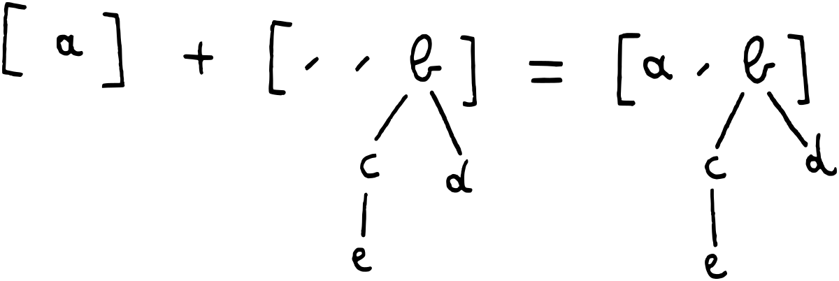
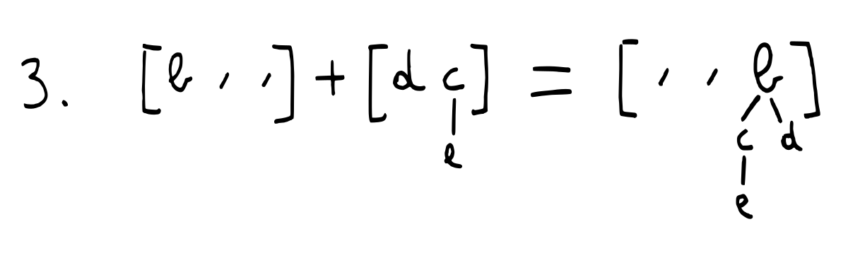
    F0 (insertTree (mergeTree l r) (mergeForests lf rf))

It’s worth seeing how the different branches in insertTree and mergeForests match up almost 1:1 with the different clauses in the definition of the type families BInc and BAdd. If we overlay them visually:

That is the intuitive explanation as to why no additional proofs or type-level trickery are required here.

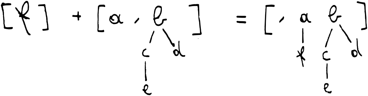
Here is an informal illustration of what happens when we don’t need to merge any trees. The singleton Forest on the left is simply put in the empty F0 spot on the right.

When there is already a tree there, we merge the trees using mergeTree and carry that, in a very similar way to how carrying works in the addition of binary numbers:

The binomial heap

The Forest structure is the main workhorse and Heap is just a simple wrapper on top of that, where we start out with a tree of order 0:

newtype Heap (b :: Binary) a = Heap {unHeap :: Forest 'Zero b a}

The operations on Heap are also simple wrappers around the previously defined functions:

emptyHeap :: Heap 'BEnd a
emptyHeap = Heap emptyForest

pushHeap :: Ord a => a -> Heap b a -> Heap (BInc b) a
pushHeap x (Heap forest) = Heap (insertTree (singletonTree x) forest)

mergeHeap :: Ord a => Heap lb a -> Heap rb a -> Heap (BAdd lb rb) a
mergeHeap (Heap lf) (Heap rf) = Heap (mergeForests lf rf)

We are now ready to show this off in GHCi again:

*Main> :t pushHeap 'a' $ pushHeap 'b' $ pushHeap 'c' $
            pushHeap 'd' $ pushHeap 'e' emptyHeap
Heap ('B1 ('B0 ('B1 'BEnd))) Char

We can also take a look at the internals of the datastructure using a custom show instance provided in the appendix 2:

*Main> pushHeap 'a' $ pushHeap 'b' $ pushHeap 'c' $
            pushHeap 'd' $ pushHeap 'e' emptyHeap
(tree of order 0)
 'a'
(no tree of order 1)
(tree of order 2)
 'b'
  'd'
   'e'
  'c'

Neat!

Binomial heaps: let’s break it down

I think it’s interesting that we have implemented an append-only heap without even requiring any lemmas so far. It is perhaps a good illustration of how append-only datastructures are conceptually much simpler.

Things get significantly more complicated when we try to implement popping the smallest element from the queue. For reference, I implemented the current heap in a couple of hours, whereas I worked on the rest of the code on and off for about a week.

Let’s look at a quick illustration of how popping works.

We first select the tree with the smallest root and remove it from the heap:

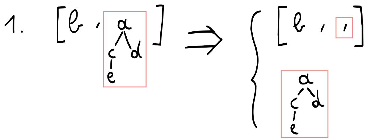
We break up the tree we selected into its root (which will be the element that is “popped”) and its children, which we turn into a new heap.

We merge the remainder heap from step 1 together with the new heap we made out of the children of the removed tree:

The above merge requires carrying twice.

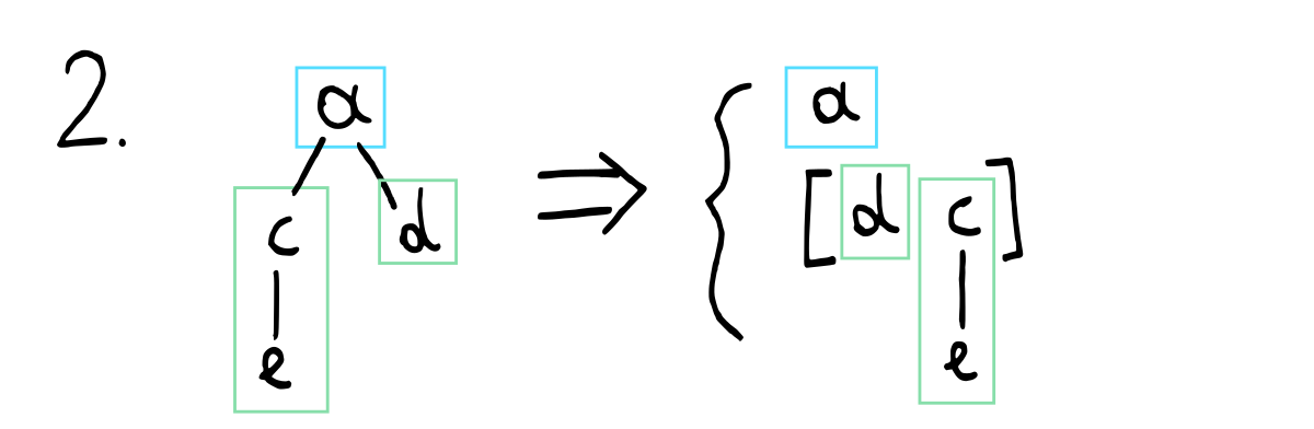
Taking apart a single tree

We will start by implementing step 2 of the algorithm above since it is a bit easier. In this step, we are taking all children from a tree and turning that into a new heap.

We need to keep all our invariants intact, and in this case this means tracking them in the type system. A tree of k has 2ᵏ elements. If we remove the root, we have k children trees with 2ᵏ - 1 elements in total. Every child becomes a tree in the new heap. This means that the heap contains k full trees, and its shape will be written as k “1”s. This matches our math: if you write k “1”s, you get the binary notation of 2ᵏ - 1.

Visually:

We introduce a type family for computing n “1”s:

type family Ones (n :: Nat) :: Binary where
    Ones 'Zero     = 'BEnd
    Ones ('Succ n) = 'B1 (Ones n)

We will use a helper function childrenToForest_go to maintain some invariants. The wrapper childrenToForest is trivially defined but its type tells us a whole deal:

childrenToForest
    :: Children n a
    -> Forest 'Zero (Ones n) a
childrenToForest children =
    childrenToForest_go SZero (childrenSingleton children) FEnd children

We use childrenSingleton to obtain a singleton for n.

childrenSingleton :: Children n a -> SNat n
childrenSingleton CZero       = SZero
childrenSingleton (CCons _ c) = SSucc (childrenSingleton c)

The tricky bit is that the list of trees in Children has them in descending order, and we want them in ascending order in Forest. This means we will have to reverse the list.

We can reverse a list easily using an accumulator in Haskell. In order to maintain the type invariants at every step, we will increase the size of the accumulator as we decrease the size of the children. This can be captured by requiring that their sum remains equal (m ~ NAdd x n).

childrenToForest_go
    :: m ~ NAdd x n
    => SNat x
    -> SNat n
    -> Forest n (Ones x) a
    -> Children n a
    -> Forest 'Zero (Ones m) a

childrenToForest_go xnat _snat@SZero acc CZero =

I will not always go into detail on how the lemmas apply but let’s do it here nonetheless.

For the base case, we simply want to return our accumulator. However, our accumulator has the type Forest n (Ones x) and we expect something of the type Forest n (Ones m). Furthermore, we know that:

  n ~ 'Zero, m ~ NAdd x n
⊢ m ~ NAdd x 'Zero

We need to prove that x ~ m in order to do the cast from Forest n (Ones x) to Forest n (Ones m).

We can do so by applying lemma1 to x (the latter represented here by xnat). This gives us lemma1 xnat :: NAdd x 'Zero :~: n. Combining this with what we already knew:

  m ~ NAdd x 'Zero, NAdd x 'Zero ~ n
⊢ m ~ x

…which is what we needed to know.

    case lemma1 xnat of QED -> acc

The inductive case is a bit harder and requires us to prove that:

  m ~ NAdd x n, m ~ NAdd x n, n ~ 'Succ k
⊢ Ones m ~ 'B1 (Ones (NAdd x k))

GHC does a great job and ends up with something like:

Ones (NAdd x (Succ k)) ~ 'B1 (Ones (NAdd x k))

Which only requires us to prove commutativity on NAdd. You can see that proof in lemma2 a bit further below. This case also illustrates well how we carry around the singletons as inputs for our lemmas and call on them when required.

childrenToForest_go xnat (SSucc nnat) acc (CCons tree children) =
    case lemma2 xnat nnat of
        QED -> childrenToForest_go
            (SSucc xnat)
            nnat
            (F1 tree acc)
            children

Proving lemma2 is trivial… once you figure out what you need to prove and how all of this works.

It took me a good amount of time to put the different pieces together in my head. It is not only a matter of proving the lemma: restructuring the code in childrenToForest_go leads to different lemmas you can attempt to prove, and figuring out which ones are feasible is a big part of writing code like this.

lemma2 :: SNat n -> SNat m -> NAdd n ('Succ m) :~: 'Succ (NAdd n m)
lemma2 SZero     _ = QED
lemma2 (SSucc n) m = case lemma2 n m of QED -> QED

More Vec utilities

These are some minor auxiliary functions we need to implement on Vec. We mention them here because we’ll also need two type classes dealing with non-zeroness.

First, we need some sort of map, and we can do this by implementing the Functor typeclass.

instance Functor (Vec n) where
    fmap _ VNull       = VNull
    fmap f (VCons x v) = VCons (f x) (fmap f v)

Secondly, we need a very simple function to convert a Vec to a list. Note that this erases the information we have about the size of the list.

vecToList :: Vec n a -> [a]
vecToList VNull       = []
vecToList (VCons x v) = x : vecToList v

Using vecToList, we can build a function to convert a non-empty Vec to a NonEmpty list. This uses an additional NNonZero typeclass.

vecToNonEmpty :: NNonZero n ~ 'True => Vec n a -> NonEmpty a
vecToNonEmpty (VCons x v) = x :| vecToList v

type family NNonZero (n :: Nat) :: Bool where
    NNonZero 'Zero     = 'False
    NNonZero ('Succ _) = 'True

Non-zeroness can be defined on binary numbers as well:

type family BNonZero (b :: Binary) :: Bool where
    BNonZero 'BEnd   = 'False
    BNonZero ('B1 b) = 'True
    BNonZero ('B0 b) = BNonZero b

You might be asking why we cannot use a simpler type, such as:

vecToNonEmpty :: Vec ('Succ n) a -> NonEmpty a

It we use this, we run into trouble when trying to prove that a Vec is not empty later on. We would have to construct a singleton for n, and we only have something that looks a bit like ∃n. 'Succ n. Trying to get the n out of that requires some form of non-zeroness constraint… which would be exactly what we are trying to avoid by using the simpler type. ⁵

Popcount and width

The minimal element will always be the root of one of our trees. That means we have as many choices for our minimal element as there are trees in our heap. We need some way to write down this number as a type.

Since we have a tree for every 1 in our binary number, we can define the number of trees as the popcount of the binary number.

In a weird twist of fate, you can also pretend this stands for “the count of trees which we can pop”, which is exactly what we will be using it for.

type family Popcount (b :: Binary) :: Nat where
    Popcount 'BEnd   = 'Zero
    Popcount ('B1 b) = 'Succ (Popcount b)
    Popcount ('B0 b) = Popcount b

Popcount can be used to relate the non-zeroness of a natural number, and the non-zeroness of a binary number.

lemma3
    :: BNonZero b ~ 'True
    => SBin b
    -> NNonZero (Popcount b) :~: 'True
lemma3 (SB1 _) = QED
lemma3 (SB0 b) = case lemma3 b of QED -> QED

In addition to caring about the popcount of a binary number, we are sometimes interested in its width (number of bits). This is also easily captured in a type family:

type family Width (binary :: Binary) :: Nat where
    Width 'BEnd        = 'Zero
    Width ('B0 binary) = 'Succ (Width binary)
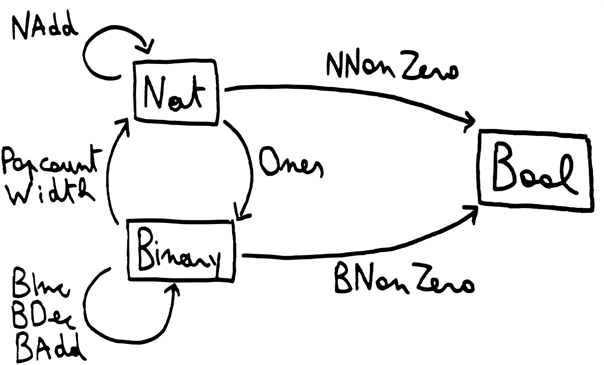
    Width ('B1 binary) = 'Succ (Width binary)

That is a fair amount of type families so far. To make things a bit more clear, here is an informal visual overview of all the type families we have defined, including BDec (binary decrement, defined further below).

Lumberjack

Now, popping the smallest element from the heap first involves cutting a single tree from the forest inside the heap. We take the root of that tree and merge the children of the tree back together with the original heap.

However, just selecting (and removing) a single tree turns out to be quite an endeavour on its own. We define an auxiliary GADT which holds the tree, the remainder of the heap, and most importantly, a lot of invariants.

Feel free to scroll down to the datatype from here if you are willing to assume the specific constraint and types are there for a reason.

The two first fields are simply evidence singletons that we carry about. k stands for the same concept as in Forest; it means we are starting with an order of k. x stands for the index of the tree that was selected.

This means the tree that was selected has an order of NAdd k x, as we can see in the third field. If the remainder of the heap is Forest k b a, its shape is denoted by b and we can reason about the shape of the original heap.

The children of tree (Tree (NAdd k x) a) that was selected will convert to a heap of shape Ones x. We work backwards from that to try and write down the type for the original heap. The tree (Tree (NAdd k x) a) would form a singleton heap of shape BInc (Ones x). The remainder (i.e., the forest with this tree removed) had shape b, so we can deduce that the original shape of the forest must have been BAdd b (BInc (Ones x)).

Finally, we restructure the type in that result to BInc (BAdd b (Ones x)). The restructuring is trivially allowed by GHC since it just requires applying the necessary type families. The restructured type turns out to be more easily usable in the places where we case-analyse CutTree further down in this blogpost.

We also carry a constraint here that seems very arbitrary and relates the widths of two binary numbers. It is easier to understand from an intuitive point of view: the new (merged) heap has the same width as the original heap. Why is it here?

Well, it turns out we will need this fact further down in a function definition. If we can conclude it here by construction in the GADT, we avoid having to prove it further down.

Of course, I know that I will need this further down because I already have the code compiling. When writing this, there is often a very, very painful dialogue in between different functions and datatypes, where you try to mediate by making the requested and expected types match by bringing them closer together step by step. In the end, you get a monstrosity like:

data CutTree (k :: Nat) (b :: Binary) a where
    CutTree
        :: Width (BAdd b (Ones x)) ~ Width (BInc (BAdd b (Ones x)))
        => SNat x
        -> SNat k
        -> Tree (NAdd k x) a
        -> Forest k b a
        -> CutTree k (BInc (BAdd b (Ones x))) a

Fortunately, this type is internal only and doesn’t need to be exported.

lumberjack_go is the worker function that takes all possible trees out of a heap. For every 1 in the shape of the heap, we have a tree: therefore it should not be a surprise that the length of the resulting vector is Popcount b.

lumberjack_go
    :: forall k b a.
       SNat k
    -> Forest k b a
    -> Vec (Popcount b) (CutTree k b a)

The definition is recursive and a good example of how recursion corresponds with inductive proofs (we’re using lemma1 and lemma2 here). We don’t go into much detail with our explanation here – this code is often hard to write, but surprisingly easy to read.

lumberjack_go _ FEnd = VNull
lumberjack_go nnat0 (F0 forest0) = fmap
    (\cutTree -> case cutTree of
        CutTree xnat (SSucc nnat) t1 forest1 -> CutTree
            (SSucc xnat)
            nnat
            (case lemma2 nnat xnat of QED -> t1)
            (F0 forest1))
    (lumberjack_go (SSucc nnat0) forest0)
lumberjack_go nnat0 (F1 tree0 forest0) = VCons
    (CutTree
        SZero
        nnat0
        (case lemma1 nnat0 of QED -> tree0)
        (F0 forest0))
    (fmap
        (\cutTree -> case cutTree of
            CutTree xnat (SSucc nnat) t1 forest1 -> CutTree
                (SSucc xnat)
                nnat
                (case lemma2 nnat xnat of QED -> t1)
                (F1 tree0 forest1))
        (lumberjack_go (SSucc nnat0) forest0))

Lumberjack: final form

Now that we can select Popcount b trees, it’s time to convert this to something more convenient to work with. We will use a NonEmpty to represent our list of candidates to select from.

lumberjack
    :: forall b a. BNonZero b ~ 'True
    => Forest 'Zero b a
    -> NonEmpty.NonEmpty (CutTree 'Zero b a)

First, we select the Popcount b trees:

lumberjack trees =
    let cutTrees :: Vec (Popcount b) (CutTree 'Zero b a)
        cutTrees = lumberjack_go SZero trees in

Then we convert it to a NonEmpty. This requires us to call lemma3 (the proof that relates non-zeroness of a binary number with non-zeroness of a natural number through popcount). We need an appropriate SBin to call lemma3 and the auxiliary function forestSingleton defined just below does that for us.

    case lemma3 (forestSingleton trees :: SBin b) of
         QED -> vecToNonEmpty cutTrees

This function is similar to childrenSingleton – it constructs an appropriate singleton we can use in proofs.

forestSingleton :: Forest k b a -> SBin b
forestSingleton FEnd     = SBEnd
forestSingleton (F0 t)   = SB0 (forestSingleton t)
forestSingleton (F1 _ t) = SB1 (forestSingleton t)

popHeap: gluing the pieces together

We can now find all trees in the heap that may be cut. They are returned in a CutTree datatype. If we assume that we are taking a specific CutTree, we can take the root from the tree inside this datatype, and we can construct a new heap from its children using childrenToForest. Then, we merge it back together with the original heap.

The new heap has one less element – hence we use BDec (binary decrement, defined just a bit below).

popForest
    :: forall a b. Ord a
    => CutTree 'Zero b a
    -> (a, Forest 'Zero (BDec b) a)

We deconstruct the CutTree to get the root (x) of the selected tree, the children of the selected trees (children), and the remaining trees in the heap (forest).

popForest (CutTree
            _xnat _nnat
            (Tree x (children :: Children r a))
            (forest :: Forest 'Zero l a)) =

We construct a new forest from the children.

    let cforest = childrenToForest children

We merge it with the remainder of the heap:

        merged :: Forest 'Zero (BAdd l (Ones r)) a
        merged = mergeForests forest cforest

The illustration from above applies here:

Now, we cast it to the result using a new lemma4 with a singleton that we construct from the trees:

        evidence :: SBin (BAdd l (Ones r))
        evidence = forestSingleton merged in
    (x, case lemma4 evidence of QED -> merged)

This is the type family for binary decrement. It is partial, as expected – you cannot decrement zero. This is a bit unfortunate but necessary. Having the BNonZero type family and using it as a constraint will solve that though.

type family BDec (binary :: Binary) :: Binary where
    BDec ('B1 b) = 'B0 b
    BDec ('B0 b) = 'B1 (BDec b)

The weirdly specific lemma4 helps us prove that we can take a number, increment it and then decrement it, and then get the same number back provided incrementing doesn’t change its width. This ends up matching perfectly with the width constraint generated by the CutTree, where the number that we increment is a number of “1”s smaller than the shape of the total heap (intuitively).

Using another constraint in CutTree with another proof here should also be possible. I found it hard to reason about why this constraint is necessary, but once I understood that it wasn’t too abnormal. The proof is easy though.

lemma4
    :: (Width x ~ Width (BInc x))
    => SBin x
    -> BDec (BInc x) :~: x
lemma4 (SB0 _) = QED
lemma4 (SB1 b) = case lemma4 b of QED -> QED

We don’t need to define a clause for SBEnd since Width SBEnd ~ Width (BInc SBEnd) does not hold.

Tying all of this together makes for a relatively easy readable popHeap:

popHeap
    :: (BNonZero b ~ 'True, Ord a)
    => Heap b a -> (a, Heap (BDec b) a)
popHeap (Heap forest0) =

Out of the different candidates, select the one with the minimal root (minimumBy is total on NonEmpty):

    let cutTrees = lumberjack forest0
        selected = minimumBy (comparing cutTreeRoot) cutTrees in

Pop that tree using popForest:

    case popForest selected of
        (x, forest1) -> (x, Heap forest1)

Helper to compare candidates by root:

  where
    cutTreeRoot :: CutTree k b a -> a
    cutTreeRoot (CutTree _ _ (Tree x _) _) = x

In GHCi:

*Main> let heap = pushHeap 'a' $ pushHeap 'b' $ pushHeap 'c' $
                pushHeap 'd' $ pushHeap 'e' emptyHeap
*Main> :t heap
heap :: Heap ('B1 ('B0 ('B1 'BEnd))) Char
*Main> :t popHeap heap
popHeap heap :: (Char, Heap ('B0 ('B0 ('B1 'BEnd))) Char)
*Main> fst $ popHeap heap
'a'
*Main> snd $ popHeap heap
(no tree of order 0)
(no tree of order 1)
(tree of order 2)
 'b'
  'd'
   'e'
  'c'

Beautiful! Our final interface to deal with the heap looks like this:

emptyHeap
    :: Heap ('B0 'BEnd) a
pushHeap
    :: Ord a
    => a -> Heap b a -> Heap (BInc b) a
mergeHeap
    :: Ord a
    => Heap lb a -> Heap rb a -> Heap (BAdd lb rb) a
popHeap
    :: (BNonZero b ~ 'True, Ord a)
    => Heap b a -> (a, Heap (BDec b) a)

Acknowledgements

I would like to thank Alex Lang for many discussions about this and for proofreading, Akio Takano and Fumiaki Kinoshita for some whiteboarding, and Titouan Vervack and Becki Lee for many additional corrections.

I am by no means an expert in dependent types so while GHC can guarantee that my logic is sound, I cannot guarantee that my code is the most elegant or that my explanations are waterproof. In particular, I am a bit worried about the fact that binary numbers do not have unique representations – even though it does seem to make the code a bit simpler. If you have any ideas for improvements, however, feel free to reach out!

Update: Lars Brünjes contacted me and showed me a similar implementation he did for leftist heaps. You can see it in this repository. He uses a similar but unique representation of binary numbers, along the lines of:

data Binary   = Zero | StrictlyPositive Positive
data Positive = B1End | B0 Positive | B1 Positive

I think this is actually more elegant than the representation I used. The only disadvantage is that is a bit less concise (which is somewhat relevant for a blogpost), requiring two functions and two datatypes for most cases (e.g. a Forest k Binary and a PForest k Positive, with mergeForests and mergePForests, and so on). But if you wanted to use this idea in a real implementation, I encourage you to check that out.

Appendices

Appendix 1: runtime cost of this approach

Since we represent the proofs at runtime, we incur an overhead in two ways:

• Carrying around and allocating the singletons;
• Evaluating the lemmas to the QED constructor.

It should be possible to remove these at runtime once the code has been typechecked, possibly using some sort of GHC core or source plugin (or CPP in a darker universe).

Another existing issue is that the tree of the spine is never “cleaned up”. We never remove trailing F0 constructors. This means that if you fill a heap of eight elements and remove all of them again, you will end up with a heap with zero elements that has the shape 'B0 ('B0 ('B0 ('B0 'BEnd))) rather than B0 'BEnd. However, this sufficed for my use case. It should be possible to add and prove a clean-up step, but it’s a bit outside the scope of this blogpost.

Appendix 2: “pretty”-printing of heaps

instance forall a b. Show a => Show (Heap b a) where
    show = intercalate "\n" . goTrees 0 . unHeap
      where
        goTrees :: forall m c. Show a => Int -> Forest m c a -> [String]
        goTrees _ FEnd = []
        goTrees order (F0 trees) =
            ("(no tree of order " ++ show order ++ ")") :
            goTrees (order + 1) trees
        goTrees order (F1 tree trees) =
            ("(tree of order " ++ show order ++ ")") :
            goTree " " tree ++
            goTrees (order + 1) trees

        goTree :: forall m. String -> Tree m a -> [String]
        goTree indentation (Tree x children) =
            (indentation ++ show x) :
            goChildren (' ' : indentation) children

        goChildren :: forall m. String -> Children m a -> [String]
        goChildren _           CZero        = []
        goChildren indentation (CCons x xs) =
            goTree indentation x ++ goChildren indentation xs

Appendix 3: left-to-right increment

Increment gets tricky mainly because we need some way to communicate the carry back in a right-to-left direction. We can do this with a type-level Either and some utility functions. It’s not too far from what we would write on a term-level, but again, a bit more clunky. We avoid this kind of clunkiness since having significantly more code obviously requires significantly more proving.

type family BIncLTR (b :: Binary) :: Binary where
    BIncLTR b = FromRight 'B1 (Carry b)

type family Carry (b :: Binary) :: Either Binary Binary where
    Carry ('B1 'BEnd) = 'Left ('B0 'BEnd)
    Carry ('B0 'BEnd) = 'Right ('B1 'BEnd)
    Carry ('B0 b)     = 'Right (UnEither 'B1 'B0 (Carry b))
    Carry ('B1 b)     = MapEither 'B0 'B1 (Carry b)

type family MapEither
        (f :: a -> c) (g :: b -> d) (e :: Either a b) :: Either c d where
    MapEither f _ ('Left x)  = 'Left (f x)
    MapEither _ g ('Right y) = 'Right (g y)

type family UnEither
        (f :: a -> c) (g :: b -> c) (e :: Either a b) :: c where
    UnEither f _ ('Left x)  = f x
    UnEither _ g ('Right y) = g y

type family FromRight (f :: a -> b) (e :: Either a b) :: b where
    FromRight f ('Left x) = f x
    FromRight _ ('Right y) = y