Parallelizing a nonogram solver
Published on July 5, 2011 under the tag haskell
What is this?
I took a course on programming languages at Ghent University this year, and a part of our assignment focused on creating and parallelizing a nonogram solver in a declarative language – where Haskell was categorized as a declarative language, because of it’s referential transparency.
If you don’t know what a nonogram is (I didn’t), you can find a really good explanation (including an animation) on the Wikipedia page.
This blogpost contains the code and report as literate Haskell. It should run
and compile, however, I have not included the example inputs here. You can find
these in the repo, under assignment-2. What follows below is the blogified
version of my report (raw version here).
Choice of programming language
I chose to implement the nonogram solver in the Haskell programming language. Haskell was chosen for a number of reasons:
- availability of a high-performance compiler, GHC;
- good Literate Programming support;
- semi-implicit parallelization using annotations;
- referential transparency which allows a more declarative programming model.
Implementation
The sequential and parallel nonogram solvers are implemented in the
Nonogram.lhs file. This is a literate Haskell file containing the report as
well as the carefully explained source code.
The Main.hs file has an entry point for an executable to solve a puzzle
concurrently, and a simple parser for a standard nonogram file format.
We can compile and run the program like this:
$ make
ghc --make -O2 -threaded Main.hs -o nonogram-solver
[1 of 1] Compiling Nonogram         ( Nonogram.lhs, Nonogram.o )
[2 of 2] Compiling Main             ( Main.hs, Main.o )
Linking nonogram-solver ...
$ ./nonogram-solver 20x20.nonogram
Parsing 20x20.nonogram
Solving 20x20.nonogram
----------XXX-------
---------XXXXX------
---------XXX-X------
---------XX--X------
------XXX-XXX-XXXX--
----XX--XX---XXXXXXX
--XXXXXX-X---X------
-XXXX---XX--XX------
--------X---X-------
-------XXX--X-------
-------XXXXXX-------
-XX---XXXXXXX-------
XXXXXX--XXX-X-------
X-XX--XX-X--X-------
---XXXX--X-X--XXX---
--------XXXX-XX-XX--
--------XXX--XXX-X--
-------XXX----XXX---
------XXX-----------
------XX-X----------
Note that you might need to install the parallel package, for example using
cabal-install. The parallel package is based on the Algorithm + Strategy =
Parallelism paper and gives us a high-level interface to add parallelism to
our program.
Parallelization conclusions
We can now compare the performance of the sequential program to the performance
of the parallel program. We use the excellent criterion library, aimed at
benchmarking Haskell code. The code we used to benchmark the the programs is
located in the Benchmark.hs file, along with some sample puzzles. To
reproduce the benchmarks, the Makefile contains the benchmark-sequential and
benchmark-parallel targets, which benchmark the sequential and parallel
program.
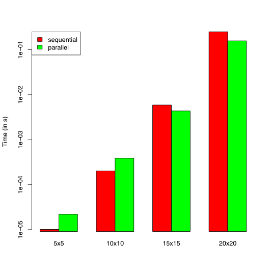
We ran these benchmarks on an Intel(R) Core(TM)2 Duo CPU E8400 @ 3.00GHz. Because we use a dual-core computer, we can at most expect a 100% speedup (i.e. a reduction of the running time by 50%).
| 5x5 | 10x10 | 15x15 | 20x20 | |
|---|---|---|---|---|
| sequential | 10.10453 us | 202.7505 us | 5.911520 ms | 250.8528 ms |
| parallel | 22.05260 us | 392.9396 us | 4.348415 ms | 155.6637 ms |
Looking at the results, parallelization introduces a large overhead for the
smaller puzzles, but gives us an advantage for larger puzzles. Because of our
implementation of the branch-and-bound-based algorithm, we know that for each
branch, a par call is made. However, this is only useful if the branch is a
non-trivial computation: otherwise, the overhead of the par call outweighs the
benefits of parallelization. We can conclude that the parallelization for this
algorithm is only useful for large enough input sets: otherwise, the overhead
outweighs the speedup.
For the 20x20 puzzle, we see that the running time is reduced by 37.9461%. This is not the 50% reduction we were naively hoping for, but it is not a bad result, since the parallelization of the program was almost trivial (just replacing the branching function). We also have to keep in mind that not everything can happen in parallel: e.g. joining the results of two branches happens on one core.
Literate source code
Here, we give the full source code to the programs, annotated in Literate Programming style.
module Nonogram
    ( Description
    , sequentialNonogram
    , parallelNonogram
    , putNonogram
    ) where

import Control.Monad (when, mplus, foldM)
import Control.Parallel (par, pseq)
import Data.IntMap (IntMap)
import qualified Data.IntMap as IM
A nonogram grid is built from cells in two possible colors. For representing the
value of a cell, we use a simple datatype called Color.
data Color = White | Black
           deriving (Show, Eq)
A nonogram is then defined as a matrix of colors:
type Nonogram = [[Color]]The input is a list of natural numbers for every row and column. We call such a
list a Description and represent it as an Int list:
type Description = [Int]We use an algorithm that attempts to solve the puzzle top-down, i.e. starting at the top row and finishing at the bottom row. It is implemented as a branch-and-bound algorithm, searching the solution space.
As we solve more and more rows, we also learn new, partial information about the
columns – in addition to the Description of the columns. We use this to
“bound” in certain cases, if the current search space does not match our partial
information.
data Partial = MustBe Color
             | BlackArea Int
             deriving (Show, Eq)
Initially, this partial information is deduced from the descriptions alone.
Hence, we have a function to convert a Description into Partial information.
fromDescription :: Description -> [Partial]
fromDescription = map BlackArea
When we reach the bottom of the nonogram, we will have a “final state” of the
partials for every column. We then need to check if we “used up” all black
areas: this function checks if the partial information can be considered empty.
Note that we do allow White fields in empty partials (since they do not add to
the description counts).
emptyPartial :: [Partial] -> Bool
emptyPartial [] = True
emptyPartial (MustBe Black : _) = False
emptyPartial (BlackArea _ : _) = False
emptyPartial (_ : xs) = emptyPartial xs
We need to keep a [Partial] for every column. We can’t store them in a list
because we want fast random access. We use an IntMap, a purely functional
tree-like structure (big-endian patricia trees) which performs fast for lookups
and insertions.
type Partials = IntMap [Partial]The following function adds a cell to partial information. It returns a value in
the Maybe monad:
if the cell is inconsistent with previous information, it returns
Nothing;otherwise, it returns the updated partial information.
On update, it might consume or add to the partial information. Note that the partial information always represents “what comes next” in the column, so we only need to inspect/modify the first few elements of the list.
learnCell :: Color -> [Partial] -> Maybe [Partial]
learnCell White [] = Just []
learnCell Black [] = Nothing
learnCell y (MustBe x : ds) = if x == y then Just ds else Nothing
learnCell White ds = Just ds
learnCell Black (BlackArea n : ds) = Just $
    replicate (n - 1) (MustBe Black) ++ (MustBe White : ds)
We also provide a convenience function to call learnCell for a particular
column (specified by it’s 0-based index).
learnCellAt :: Color -> Partials -> Int -> Maybe Partials
learnCellAt cell partials index = do
    ds <- learnCell cell $ partials IM.! index
    return $ IM.insert index ds partials
In Haskell, we can abstract over pretty much anything. We need to write two versions of our nonogram solving algorithm – a simple one and a concurrent one. Since we want as little code duplication as possible, we can do this by abstracting over the way we deal with branches in our search tree.
More concrete, we have a branching strategy (Branching) which decides how two
branches which might or might not yield a result (the Maybe a’s) are composed.
We also provide sequential and parallel branching:
type Branching a = Maybe a -> Maybe a -> Maybe asequential :: Branching a
sequential = mplusparallel :: Branching a
parallel x y = x `par` y `pseq` mplus x yParallelization of Haskell programs can be easily done using par annotations,
which attempts to spark the calculation of a thunk on a free core (if possible).
While par is a very cheap function call, it is not free. Therefore, one
always has to make sure the computations we spark on other cores are big enough,
so we minimize the overhead caused by par.
This implies it could be a better strategy to only use parallel branching if we
are in the upper part of the search tree (i.e. depth is less than a given n).
However, after experimenting with this, this n was highly dependent of the
used input set, and the speedup was only marginally better than the simpler
solution using just parallel – so I decided not to use this more advanced
strategy.
The strategy is used in the solve function, which holds most of the main
solver logic.
The solve function is actually a wrapper around a solve' function which does
the actual work. This is an optimization called the static argument
transformation.
solve :: Branching Nonogram -> Int -> Int -> [Description] -> Partials
      -> Maybe Nonogram
solve branch width = solve'
  where
    solve' column descriptions partials
There are a number of cases that need to be considered. First, suppose there are
no more descriptions for the rows. In this case, we know that the knowledge we
have about the column partials must be empty: we can no longer place any black
cells. If this is the case, we have a correct solution (the empty one),
otherwise, our solver fails by returning Nothing.
        | null descriptions =
            if all emptyPartial (map snd $ IM.toList partials)
                then return [[]]
                else Nothing
If we have at least one row description, we check to see if that row description
is empty. Suppose this is the case. This means no more black areas should be
placed in this row, so we just fill it up with white cells. We then recursively
call solve' to solve the other rows.
        | null rd = do
            ps <- foldM (learnCellAt White) partials [column .. width - 1]
            rows <- solve' 0 rds ps
            return $ replicate (width - column) White : rows
Since we know now that the row description is not empty, we have at least one black area on this row. We consider two possibilities:
- the black areas starts at the beginning of the row (consider the beginning of
the row as indicated by the
columnargument); - we have at least one white cell, followed by a row with the same black areas.
This is where our search tree branches between the two cases, branch and
skip, defined later.
| otherwise = branch place skipSome definitions of previously used values:
      where
        (rd : rds) = descriptions
        (l : ds) = rd
The case where the black area is at the beginning at the row has a pretty long definition but the logic behind the code is actually quite straightforward:
- we fail if the black area cannot be placed due to the fact there are insuficient cells left;
- we update the the column partial knowledge with these new black cells;
- we place a white cell after the black area, two because black areas cannot be contiguous (if the end of the black area touches the border of the grid, we can skip this);
- we recursively call
solve'to solve the rest of the row, then add the cells we just calculated to the returned solution.
        place = do
            when (column + l > width) Nothing
            ps <- foldM (learnCellAt Black) partials
                      [column .. column + l - 1]

            let atEnd = column + l == width

            ps' <- if atEnd then return ps
                            else learnCellAt White ps (column + l)

            (row : rows) <- solve' (column + l + 1) (ds : rds) ps'
            let row' = if atEnd then row else White : row
            return $ (replicate l Black ++ row') : rows
If we choose not to place the black area at the beginning of the row, we just
need to add a white cell and recursively call solve' again. This case can fail
as well – when we’ve reached the far right side of the grid, we can no longer
place white cells.
        skip = do
            when (column >= width) Nothing
            ps <- learnCellAt White partials column
            (row : rows) <- solve' (column + 1) ((l : ds) : rds) ps
            return $ ((White : row)) : rows
The nonogram function helps us in converting the column descriptions into the
partial information we need, and thus provides a nicer interface to the
programmer than solve does.
nonogram :: Branching Nonogram -> [Description] -> [Description]
         -> Maybe Nonogram
nonogram branch rows columns = solve branch (length columns) 0 rows state
  where
    state = IM.fromList (zip [0 ..] $ map fromDescription columns)
We provide a sequential and a parallel program:
sequentialNonogram :: [Description] -> [Description] -> Maybe Nonogram
sequentialNonogram = nonogram sequential
parallelNonogram :: [Description] -> [Description] -> Maybe Nonogram
parallelNonogram = nonogram parallelAt last, the putNonogram function allows us to print a solution we found
(of the type Maybe Nonogram) to standard output.
putNonogram :: Maybe Nonogram -> IO ()
putNonogram Nothing  = putStrLn "No solution found"
putNonogram (Just s) = mapM_ (putStrLn . concatMap showCell) s
  where
    showCell Black = "X"
    showCell White = "-"