Lazy I/O and graphs: Winterfell to King's Landing

Finding the shortest path in a lazily loaded infinite graph
Published on January 17, 2017 under the tag haskell

Introduction

This post is about Haskell, and lazy I/O in particular. It is a bit longer than usual, so I will start with a high-level overview of what you can expect:

We talk about how we can represent graphs in a “shallow embedding”. This means we will not use a dedicated Graph type and rather represent edges by directly referencing other Haskell values.
This is a fairly good match when we want to encode infinite ¹ graphs. When dealing with infinite graphs, there is no need to “reify” the graph and enumerate all the nodes and egdes – this would be futile anyway.
We discuss a Haskell implementation of shortest path search in a weighted graph that works on these infinite graphs and that has good performance characteristics.
We show how we can implement lazy I/O to model infinite graphs as pure values in Haskell, in a way that only the “necessary” parts of the graph are loaded from a database. This is done using the unsafeInterleaveIO primitive.
Finally, we discuss the disadvantages of this approach as well, and we review some of common problems associated with lazy I/O.

Let’s get to it!

As usual, this is a literate Haskell file, which means that you can just load this blogpost into GHCi and play with it. You can find the raw .lhs file here.

{-# LANGUAGE OverloadedStrings   #-}
{-# LANGUAGE ScopedTypeVariables #-}

import           Control.Concurrent.MVar (MVar, modifyMVar, newMVar)
import           Control.Monad           (forM_, unless)
import           Control.Monad.State     (State, gets, modify, runState)
import           Data.Hashable           (Hashable)
import qualified Data.HashMap.Strict     as HMS
import qualified Data.HashPSQ            as HashPSQ
import           Data.Monoid             ((<>))
import qualified Data.Text               as T
import qualified Data.Text.IO            as T
import qualified Database.SQLite.Simple  as SQLite
import qualified System.IO.Unsafe        as IO

The problem at hand

As an example problem, we will look at finding the shortest path between cities in Westeros, the fictional location where the A Song of Ice and Fire novels (and HBO’s Game of Thrones) take place.

We model the different cities in a straightforward way. In addition to a unique ID used to identify them, they also have a name, a position (X,Y coordinates) and a list of reachable cities, with an associated time (in days) it takes to travel there. This travel time, also referred to as the cost, is not necessarily deducable from the sets of X,Y coordinates: some roads are faster than others.

type CityId = T.Text

data City = City
    { cityId         :: CityId
    , cityName       :: T.Text
    , cityPos        :: (Double, Double)
    , cityNeighbours :: [(Double, City)]
    }

Having direct access to the neighbouring cities, instead of having to go through CityIds both has advantages and disadvantages.

On one hand, updating these values becomes cumbersome at best, and impossible at worst. If we wanted to change a city’s name, we would have to traverse all other cities to update possible references to the changed city.

On the other hand, it makes access more convenient (and faster!). Since we want a read-only view on the data, it works well in this case.

Getting the data

We will be using data extracted from got.show, conveniently licensed under a Creative Commons license. You can find the complete SQL dump here. The schema of the database should not be too surprising:

CREATE TABLE cities (
  id   text  PRIMARY KEY NOT NULL,
  name text  NOT NULL,
  x    float NOT NULL,
  y    float NOT NULL
);
CREATE TABLE roads (
  origin      text  NOT NULL,
  destination text  NOT NULL,
  cost        float NOT NULL,
  PRIMARY KEY (origin, destination)
);
CREATE INDEX roads_origin ON roads (origin);

The road costs have been generated by multiplying the actual distances with a random number uniformly chosen between 0.6 and 1.4. Cities have been (bidirectionally) connected to at least four closest neighbours. This ensures that every city is reachable.

We will use sqlite in our example because there is almost no setup involved. You can load this database by issueing:

curl -L jaspervdj.be/files/2017-01-17-got.sql.txt | sqlite3 got.db

But instead of considering the whole database (which we’ll get to later), let’s construct a simple example in Haskell so we can demonstrate the interface a bit. We can use a let to create bindings that refer to one another easily.

test01 :: IO ()
test01 = do
    let winterfell = City "wtf" "Winterfell" (-105, 78)
          [(13, moatCailin), (12, whiteHarbor)]
        whiteHarbor = City "wih" "White Harbor" (-96, 74)
          [(15, braavos), (12, winterfell)]
        moatCailin = City "mtc" "Moat Cailin" (-104, 72)
          [(20, crossroads), (13, winterfell)]
        braavos = City "brv" "Braavos" (-43, 67)
          [(17, kingsLanding), (15, whiteHarbor)]
        crossroads = City "crs" "Crossroads Inn" (-94, 58)
          [(7, kingsLanding), (20, crossroads)]
        kingsLanding = City "kgl" "King's Landing" (-84, 45)
          [(7, crossroads), (17, kingsLanding)]

    printSolution $
        shortestPath cityId cityNeighbours winterfell kingsLanding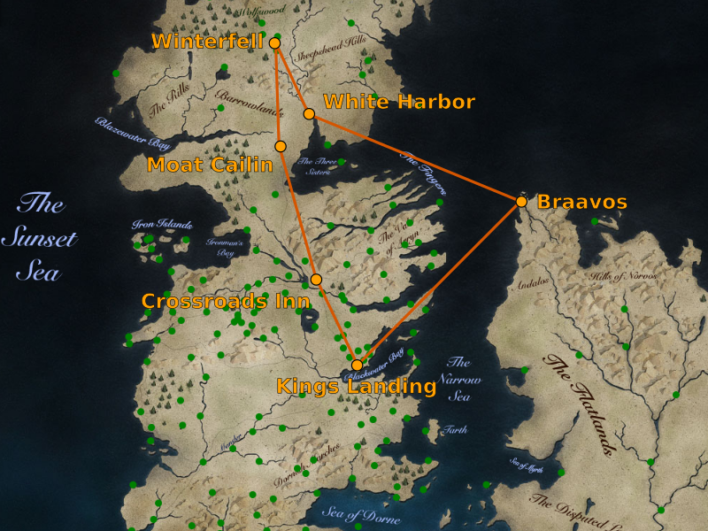

printSolution is defined as:

printSolution :: Maybe (Double, [City]) -> IO ()
printSolution Nothing             = T.putStrLn "No solution found"
printSolution (Just (cost, path)) = T.putStrLn $
    "cost: " <> T.pack (show cost) <>
    ", path: " <> T.intercalate " -> " (map cityName path)

We get exactly what we expect in GHCi:

*Main> test01
cost: 40.0, path: Winterfell -> Moat Cailin ->
Crossroads Inn -> King's Landing

So far so good! Now let’s dig in to how shortestPath works.

The Shortest Path algorithm

The following algorithm is known as Uniform Cost Search. It is a variant of Dijkstra’s graph search algorithm that is able to work with infinite graphs (or graphs that do not fit in memory anyway). It returns the shortest path between a known start and goal in a weighted directed graph.

Because this algorithm attempts to solve the problem the right way, including keeping back references, it is not simple. Therefore, if you are only interested in the part about lazy I/O, feel free to skip to this section and return to the algorithm later.

We have two auxiliary datatypes.

BackRef is a wrapper around a node and the previous node on the shortest path to the former node. Keeping these references around is necessary to iterate a list describing the entire path at the end.

data BackRef node = BackRef {brNode :: node, brPrev :: node}

We will be using a State monad to implement the shortest path algorithm. This is our state:

data SearchState node key cost = SearchState
    { ssQueue    :: HashPSQ.HashPSQ key cost (BackRef node)
    , ssBackRefs :: HMS.HashMap key node
    }

In our state, we have:

A priority queue of nodes we will visit next in ssQueue, including back references. Using a priority queue will let us grab the next node with the lowest associated cost in a trivial way.
Secondly, we have the ssBackRefs map. That one serves two purposes: to keep track of which nodes we have already explored (the keys in the map), and to keep the back references of those locations (the values in the map).

These two datatypes are only used internally in the shortestPath function. Ideally, we would be able to put them in the where clause, but that is not possible in Haskell.

Instead of declaring a Node typeclass (possibly with associated types for the key and cost types), I decided to go with simple higher-order functions. We only need two of those function arguments after all: a function to give you a node’s key (nodeKey) and a function to get the node’s neighbours and associated costs (nodeNeighbours).

shortestPath
    :: forall node key cost.
          (Ord key, Hashable key, Ord cost, Num cost)
    => (node -> key)
    -> (node -> [(cost, node)])
    -> node
    -> node
    -> Maybe (cost, [node])
shortestPath nodeKey nodeNeighbours start goal =

We start by creating an initial SearchState for our algorithm. Our initial queue holds one item (implying that we need explore the start) and our initial back references map is empty (we haven’t explored anything yet).

    let startbr      = BackRef start start
        queue0       = HashPSQ.singleton (nodeKey start) 0 startbr
        backRefs0    = HMS.empty
        searchState0 = SearchState queue0 backRefs0

walk is the main body of the shortest path search. We call that and if we found a shortest path, we return its cost together with the path which we can reconstruct from the back references (followBackRefs).

        (mbCost, searchState1) = runState walk searchState0 in
    case mbCost of
        Nothing   -> Nothing
        Just cost -> Just
            (cost, followBackRefs (ssBackRefs searchState1))
  where

Now, we have a bunch of functions that are used within the algorithm. The first one, walk, is the main body. We start by exploring the next node in the queue. By construction, this is always a node we haven’t explored before. If this node is the goal, we’re done. Otherwise, we check the node’s neighbours and update the queue with those neighbours. Then, we recursively call walk.

    walk :: State (SearchState node key cost) (Maybe cost)
    walk = do
        mbNode <- exploreNextNode
        case mbNode of
            Nothing -> return Nothing
            Just (cost, curr)
                | nodeKey curr == nodeKey goal ->
                    return (Just cost)
                | otherwise -> do
                    forM_ (nodeNeighbours curr) $ \(c, next) ->
                        updateQueue (cost + c) (BackRef next curr)
                    walk

Exploring the next node is fairly easy to implement using a priority queue: we simply need to pop the element with the minimal priority (cost) using minView. We also need indicate that we reached this node and save the back reference by inserting that info into ssBackRefs.

    exploreNextNode
        :: State (SearchState node key cost) (Maybe (cost, node))
    exploreNextNode = do
        queue0 <- gets ssQueue
        case HashPSQ.minView queue0 of
            Nothing                                   -> return Nothing
            Just (_, cost, BackRef curr prev, queue1) -> do
                modify $ \ss -> ss
                    { ssQueue    = queue1
                    , ssBackRefs =
                        HMS.insert (nodeKey curr) prev (ssBackRefs ss)
                    }
                return $ Just (cost, curr)

updateQueue is called as new neighbours are discovered. We are careful about adding new nodes to the queue:

If we have already explored this neighbour, we don’t need to add it. This is done by checking if the neighbour key is in ssBackRefs.
If the neighbour is already present in the queue with a lower priority (cost), we don’t need to add it, since we want the shortest path. This is taken care of by the utility insertIfLowerPrio, which is defined below.

    updateQueue
        :: cost -> BackRef node -> State (SearchState node key cost) ()
    updateQueue cost backRef = do
        let node = brNode backRef
        explored <- gets ssBackRefs
        unless (nodeKey node `HMS.member` explored) $ modify $ \ss -> ss
            { ssQueue = insertIfLowerPrio
                (nodeKey node) cost backRef (ssQueue ss)
            }

If the algorithm finishes, we have found the lowest cost from the start to the goal, but we don’t have the path ready. We need to reconstruct this by following the back references we saved earlier. followBackRefs does that for us. It recursively looks up nodes in the map, constructing the path in the accumulator acc on the way, until we reach the start.

    followBackRefs :: HMS.HashMap key node -> [node]
    followBackRefs paths = go [goal] goal
      where
        go acc node0 = case HMS.lookup (nodeKey node0) paths of
            Nothing    -> acc
            Just node1 ->
                if nodeKey node1 == nodeKey start
                   then start : acc
                   else go (node1 : acc) node1

That’s it! The only utility left is the insertIfLowerPrio function. Fortunately, we can easily define this using the alter function from the psqueues package. That function allows us to change a key’s associated value and priority. It also allows to return an additional result, but we don’t need that, so we just use () there.

insertIfLowerPrio
    :: (Hashable k, Ord p, Ord k)
    => k -> p -> v -> HashPSQ.HashPSQ k p v -> HashPSQ.HashPSQ k p v
insertIfLowerPrio key prio val = snd . HashPSQ.alter
    (\mbOldVal -> case mbOldVal of
        Just (oldPrio, _)
            | prio < oldPrio -> ((), Just (prio, val))
            | otherwise      -> ((), mbOldVal)
        Nothing              -> ((), Just (prio, val)))
    key

Interlude: A (very) simple cache

Lazy I/O will guarantee that we only load the nodes in the graph when necessary.

However, since we know that the nodes in the graph do not change over time, we can build an additional cache around it. That way, we can also guarantee that we only load every node once.

Implementing such a cache is very simple in Haskell. We can simply use an MVar, that will even take care of blocking ² when we have concurrent access to the cache (assuming that is what we want).

type Cache k v = MVar (HMS.HashMap k v)

newCache :: IO (Cache k v)
newCache = newMVar HMS.empty

cached :: (Hashable k, Ord k) => Cache k v -> k -> IO v -> IO v
cached mvar k iov = modifyMVar mvar $ \cache -> do
    case HMS.lookup k cache of
        Just v  -> return (cache, v)
        Nothing -> do
            v <- iov
            return (HMS.insert k v cache, v)

Note that we don’t really delete things from the cache. In order to keep things simple, we can assume that we will use a new cache for every shortest path we want to find, and that we throw away that cache afterwards.

Loading the graph using Lazy I/O

Now, we get to the main focus of the blogpost: how to use lazy I/O primitives to ensure resources are only loaded when they are needed. Since we are only concerned about one datatype (City) our loading code is fairly easy.

The most important loading function takes the SQLite connection, the cache we wrote up previously, and a city ID. We immediately use the cached combinator in the implementation, to make sure we load every CityId only once.

getCityById
    :: SQLite.Connection -> Cache CityId City -> CityId
    -> IO City
getCityById conn cache id' = cached cache id' $ do

Now, we get some information from the database. We play it a bit loose here and assume a singleton list will be returned from the query.

    [(name, x, y)] <- SQLite.query conn
        "SELECT name, x, y FROM cities WHERE id = ?" [id']

The neighbours are stored in a different table because we have a properly normalised database. We can write a simple query to obtain all roads starting from the current city:

    roads <- SQLite.query conn
        "SELECT cost, destination FROM roads WHERE origin = ?"
        [id'] :: IO [(Double, CityId)]

This leads us to the crux of the matter. The roads variable contains something of the type [(Double, CityId)], and what we really want is [(Double, City)]. We need to recursively call getCityById to load what we want. However, doing this “the normal way” would cause problems:

Since the IO monad is strict, we would end up in an infinite loop if there is a cycle in the graph (which is almost always the case for roads and cities).
Even if there was no cycle, we would run into trouble with our usage of MVar in the Cache. We block access to the Cache while we are in the cached combinator, so calling getCityById again would cause a deadlock.

This is where Lazy I/O shines. We can implement lazy I/O by using the unsafeInterleaveIO primitive. Its type is very simple and doesn’t look as threatening as unsafePerformIO.

unsafeInterleaveIO :: IO a -> IO a

It takes an IO action and defers it. This means that the IO action is not executed right now, but only when the value is demanded. That is exactly what we want!

We can simply wrap the recursive calls to getCityById using unsafeInterleaveIO:

    neighbours <- IO.unsafeInterleaveIO $
        mapM (traverse (getCityById conn cache)) roads

And then return the City we constructed:

    return $ City id' name (x, y) neighbours

Lastly, we will add a quick-and-dirty wrapper around getCityById so that we are also able to load cities by name. Its implementation is trivial:

getCityByName
    :: SQLite.Connection -> Cache CityId City -> T.Text
    -> IO City
getCityByName conn cache name = do
    [[id']] <- SQLite.query conn
        "SELECT id FROM cities WHERE name = ?" [name]
    getCityById conn cache id'

Now we can neatly wrap things up in our main function:

main :: IO ()
main = do
    cache <- newCache
    conn  <- SQLite.open "got.db"
    winterfell <- getCityByName conn cache "Winterfell"
    kings      <- getCityByName conn cache "King's Landing"
    printSolution $
        shortestPath cityId cityNeighbours winterfell kings

This works as expected:

*Main> :main
cost: 40.23610549037591, path: Winterfell -> Moat Cailin ->
Greywater Watch -> Inn of the Kneeling Man -> Fairmarket ->
Brotherhood Without Banners Hideout -> Crossroads Inn ->
Darry -> Saltpans -> QuietIsle -> Antlers -> Sow's Horn ->
Brindlewood -> Hayford -> King's Landing

Disadvantages of Lazy I/O

Lazy I/O also has many disadvantages, which have been widely discussed. Among those are:

Code becomes harder to reason about. In a setting without lazy I/O, you can casually reason about an Int as either an integer that’s already computed, or as something that will do some (pure) computation and then yield an Int.

When lazy I/O enters the picture, things become more complicated. That Int you wanted to print? Yeah, it fired a bunch of missiles and returned the bodycount.

This is why I would not seriously consider using lazy I/O when working with a team or on a large project – it can be easy to forget what is lazily loaded and what is not, and there’s no easy way to tell.
Scarce resources can easily become a problem if you are not careful. If we keep a reference to a City in our heap, that means we also keep a reference to the cache and the SQLite connection.

We must ensure that we fully evaluate the solution to something that doesn’t refer to these resources (to e.g. a printed string) so that the references can be garbage collected and the connections can be closed.

Closing the connections is a problem in itself – if we cannot guarantee that e.g. streams will be fully read, we need to rely on finalizers, which are pretty unreliable…
If we go a step further and add concurrency to our application, it becomes even tricker. Deadlocks are not easy to reason about – so how about reasoning about deadlocks when you’re not sure when the IO is going to be executed at all?

Despite all these shortcomings, I believe lazy I/O is a powerful and elegant tool that belongs in every Haskeller’s toolbox. Like pretty much anything, you need to be aware of what you are doing and understand the advantages as well as the disadvantages.

For example, the above downsides do not really apply if lazy I/O is only used within a module. For this blogpost, that means we could safely export the following interface:

shortestPathBetweenCities
    :: FilePath                       -- ^ Database name
    -> CityId                         -- ^ Start city ID
    -> CityId                         -- ^ Goal city ID
    -> IO (Maybe (Double, [CityId]))  -- ^ Cost and path
shortestPathBetweenCities dbFilePath startId goalId = do
    cache <- newCache
    conn  <- SQLite.open dbFilePath
    start <- getCityById conn cache startId
    goal  <- getCityById conn cache goalId
    case shortestPath cityId cityNeighbours start goal of
        Nothing           -> return Nothing
        Just (cost, path) ->
            let ids = map cityId path in
            cost `seq` foldr seq () ids `seq`
            return (Just (cost, ids))

Thanks for reading – and I hope I was able to offer you a nuanced view on lazy I/O. Special thanks to Jared Tobin for proofreading.

In this blogpost, I frequently talk about “infinite graphs”. Of course most of these examples are not truly infinite, but we can consider examples that do not fit in memory completely, and in that way we can regard them as “infinite for practical purposes”.↩︎
While blocking is good in this case, it might hurt performance when running in a concurrent environment. A good solution to that would be to stripe the MVars based on the keys, but that is beyond the scope of this blogpost. If you are interested in the subject, I talk about it a bit here.↩︎

Stuff

Links