Stuff

Links

Picking a random element from a frequency list

Introduction

A week or so ago, I wrote Lorem Markdownum: a small webapp to generate random text (like the many lorem ipsum generators out there), but in markdown format.

This blogpost explains a mildly interesting algorithm I used to pick a random element from a frequency list. It is written in Literate Haskell so you should be able to drop it into a file and run it – the raw version can be found here.

import           Data.List       (sortBy)
import           Data.Ord        (comparing)
import qualified Data.Map.Strict as M
import           System.Random   (randomRIO)

The problem

Lorem ipsum generators usually create random but realistic-looking text by using sample data, on which a model is trained. A very simple example of that is just to pick words according to their frequencies. Let us take some sample data from a song that fundamentally changed the music industry in the early 2000s:

Badger badger badger
Mushroom mushroom
Badger badger badger
Panic, a snake
Badger badger badger
Oh, it’s a snake!

This gives us the following frequency list:

badgers :: [(String, Int)]
badgers =
    [ ("a",        2)
    , ("badger",   9)
    , ("it's",     1)
    , ("mushroom", 2)
    , ("oh",       1)
    , ("panic",    1)
    , ("snake",    2)
    ]

The sum of all the frequencies in this list is 18. This means that we will e.g. pick “badger” with a chance of 9/18. We can naively implement this by expanding the list so it contains the items in the given frequencies and then picking one randomly.

decodeRle :: [(a, Int)] -> [a]
decodeRle []            = []
decodeRle ((x, f) : xs) = replicate f x ++ decodeRle xs

sample1 :: [(a, Int)] -> IO a
sample1 freqs = do
    let expanded = decodeRle freqs
    idx <- randomRIO (0, length expanded - 1)
    return $ expanded !! idx

This is obviously extremely inefficient, and it is not that hard to come up with a better definition: we do not expand the list, and instead use a specialised indexing function for frequency lists.

indexFreqs :: Int -> [(a, Int)] -> a
indexFreqs _   [] = error "please reboot computer"
indexFreqs idx ((x, f) : xs)
    | idx < f     = x
    | otherwise   = indexFreqs (idx - f) xs

sample2 :: [(a, Int)] -> IO a
sample2 freqs = do
    idx <- randomRIO (0, sum (map snd freqs) - 1)
    return $ indexFreqs idx freqs

However, sample2 is still relatively slow when we our sample data consists of a large amount of text (imagine what happens if we have a few thousand different words). Can we come up with a better but still elegant solution?

Note that lorem ipsum generators generally employ more complicated strategies than just picking a word according to the frequencies in the sample data. Usually, algorithms based on Markov Chains are used. But even when this is the case, picking a word with some given frequencies is still a subproblem that needs to be solved.

Frequency Trees

It is easy to see why sample2 is relatively slow: indexing in a linked list is expensive. Purely functional programming languages usually solve this by using trees instead of lists where fast indexing is required. We can use a similar approach here.

A leaf in the tree simply holds an item and its frequency. A branch also holds a frequency – namely, the sum of the frequencies of its children. By storing this computed value, we will be able to write a fast indexing this method.

data FreqTree a
    = Leaf   !Int !a
    | Branch !Int (FreqTree a) (FreqTree a)
    deriving (Show)

A quick utility function to get the sum of the frequencies in such a tree:

sumFreqs :: FreqTree a -> Int
sumFreqs (Leaf   f _)   = f
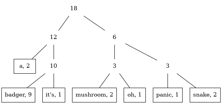
sumFreqs (Branch f _ _) = f

Let us look at the tree for badgers (we will discuss how this tree is computed later):

Once we have this structure, it is not that hard to write a faster indexing function, which is basically a search in a binary tree:

indexFreqTree :: Int -> FreqTree a -> a
indexFreqTree idx tree = case tree of
    (Leaf _ x)             -> x
    (Branch _ l r)
        | idx < sumFreqs l -> indexFreqTree idx                l
        | otherwise        -> indexFreqTree (idx - sumFreqs l) r

sample3 :: FreqTree a -> IO a
sample3 tree = do
    idx <- randomRIO (0, sumFreqs tree - 1)
    return $ indexFreqTree idx tree

There we go! We intuitively see this method is faster since we only have to walk through a few nodes – namely, those on the path from the root node to the specific leaf node.

But how fast is this, exactly? This depends on how we build the tree.

Well-balanced trees

Given a list with frequencies, we can build a nicely balanced tree (i.e., in the sense in which binary tries are balanced). This minimizes the longest path from the root to any node.

We first have a simple utility function to clean up such a list of frequencies:

uniqueFrequencies :: Ord a => [(a, Int)] -> [(a, Int)]
uniqueFrequencies =
    M.toList . M.fromListWith (+) . filter ((> 0) . snd)

And then we have the function that actually builds the tree. For a singleton list, we just return a leaf. Otherwise, we simply split the list in half, build trees out of those halves, and join them under a new parent node. Computing the total frequency of the parent node (freq) is done a bit inefficiently, but that is not the focus at this point.

balancedTree :: Ord a => [(a, Int)] -> FreqTree a
balancedTree = go . uniqueFrequencies
  where
    go []       = error "balancedTree: Empty list"
    go [(x, f)] = Leaf f x
    go xs       =
        let half     = length xs `div` 2
            (ys, zs) = splitAt half xs
            freq     = sum $ map snd xs
        in Branch freq (go ys) (go zs)

Huffman-balanced trees

However, well-balanced trees might not be the best solution for this problem. It is generally known that few words in most natural languages are extremely commonly used (e.g. “the”, “a”, or in or case, “badger”) while most words are rarely used.

For our tree, it would make sense to have the more commonly used words closer to the root of the tree – in that case, it seems intuitive that the expected number of nodes visited to pick a random word will be lower.

It turns out that this idea exactly corresponds to a Huffman tree. In a Huffman tree, we want to minimize the expected code length, which equals the expected path length. Here, we want to minimize the expected number of nodes visited during a lookup – which is precisely the expected path length!

The algorithm to construct such a tree is surprisingly simple. We start out with a list of trees: namely, one singleton leaf tree for each element in our frequency list.

Then, given this list, we take the two trees which have the lowest total sums of frequencies (sumFreqs), and join these using a branch node. This new tree is then inserted back into the list.

This algorithm is repeated until we are left with only a single tree in the list: this is our final frequency tree.

huffmanTree :: Ord a => [(a, Int)] -> FreqTree a
huffmanTree = go . map (\(x, f) -> Leaf f x) . uniqueFrequencies
  where
    go trees = case sortBy (comparing sumFreqs) trees of
        []             -> error "huffmanTree: Empty list"
        [ft]           -> ft
        (t1 : t2 : ts) ->
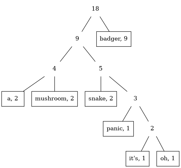
            go $ Branch (sumFreqs t1 + sumFreqs t2) t1 t2 : ts

This yields the following tree for our example:

Is the second approach really better?

Although Huffman trees are well-studied, for our example, we only intuitively explained why the second approach is probably better. Let us see if we can justify this claim a bit more, and find out how much better it is.

The expected path length L of an item in a balanced tree can be very easily approached, since it is just a binary tree and we all know those (suppose N is the number of unique words):

However, if we have a tree we built using the huffmanTree, it is not that easy to calculate the expected path length. We know that for a Huffman tree, the path length should approximate the entropy, which, in our case, gives us an approximation for the path length for item with a specified frequency f:

Where F is the total sum of all frequencies. If we assume that we know the frequency for every item, the expected path length is simply a weighted mean:

This is where it gets interesting. It turns out that the frequency of words in a natural language is a well-researched topic, and predicted by something called Zipf’s law. This law tells us that the frequency of an item f can be estimated by:

Where s characterises the distribution and is typically very close to 1 for natural languages. H is the generalised harmonic number:

If we substitute in the definition for the frequencies into the formula for the expected path length, we get:

This is something we can work with! If we plot this for s = 1, we get:

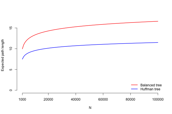
It is now clear that the expected path length for a frequency tree built using huffmanTree is expected to be significantly shorter than a frequency tree built using balancedTree, even for relatively small N. Yay! Since the algorithm now works, the conclusion is straightforward.

Conclusion

Lorem markdownum constitit foret tibi Phoebes propior poenam. Nostro sub flos auctor ventris illa choreas magnis at ille. Haec his et tuorum formae obstantes et viribus videret vertit, spoliavit iam quem neptem corpora calidis, in. Arcana ut puppis, ad agitur telum conveniant quae ardor? Adhuc arcu acies corpore amplexans equis non velamina buxi gemini est somni.

Thanks to Simon Meier, Francesco Mazzoli and some other people at Erudify for the interesting discussions about this topic!